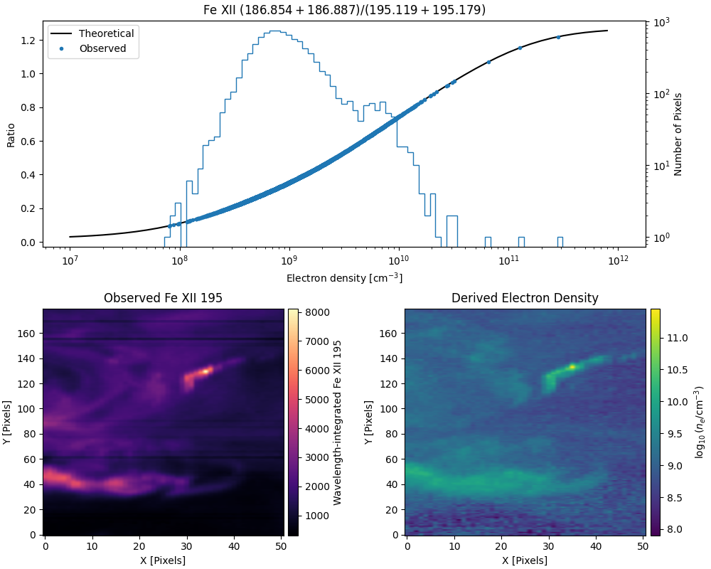
Fe XII Density Diagnostics with EIS Data

This example shows how to compute a density diagnostic from Hinode/EIS data using fiasco by reproducing some components of Fig. 7 from Mulay et al. [MZM17].

The exact density values differ from the paper because this example uses the current CHIANTI database through fiasco, together with precomputed EIS products generated from reprocessed data.

import astropy.units as u
import matplotlib.pyplot as plt
import numpy as np

from astropy.io import fits
from astropy.visualization import quantity_support

import fiasco

quantity_support()

<astropy.visualization.units.quantity_support.<locals>.MplQuantityConverter object at 0x7ae78f354230>

First download and read in the precomputed EIS products. These two FITS files are hosted in a separate data repository so that this example does not need to run the EIS fitting step with eispac. The intensity maps include the wavelength-integrated Fe XII 195 Å intensity and the fitted Fe XII 186 Å and 195 Å peak intensity.

data_base_url = 'https://media.githubusercontent.com/media/sunpy/data/main/fiasco'
with fits.open(f'{data_base_url}/jet_footpoint_fe12_observed.fits') as observed_hdul:
    integrated_195 = observed_hdul['OBSERVED_195'].data
with fits.open(f'{data_base_url}/jet_footpoint_fe12_intensities.fits') as intensity_hdul:
    intensity_186 = intensity_hdul['INTENSITY_186'].data
    intensity_195 = intensity_hdul['INTENSITY_195'].data
    intensity_header = intensity_hdul['INTENSITY_195'].header

Compute the theoretical Fe XII density-sensitive ratio curve at the temperature at which the ionization fraction of Fe XII is highest.

density = 10**np.arange(7, 12, 0.1) * u.cm**-3
fe12 = fiasco.Ion('Fe XII', 1.43 * u.MK)
ratio_curve = fiasco.line_ratio(
    fe12,
    [186.854, 186.887] * u.angstrom,
    [195.119, 195.179] * u.angstrom,
    density,
    use_two_ion_model=False,
).squeeze()

Map the observed Fe XII intensity ratio onto the theoretical curve to derive the density map.

observed_ratio = np.divide(
    intensity_186,
    intensity_195,
    out=np.full_like(intensity_186, np.nan),
    where=intensity_195 > 0,
)
density_map = np.interp(observed_ratio, ratio_curve, density, left=np.nan, right=np.nan)

Plot the theoretical ratio curve, the observed Fe XII map, and the derived density map for the jet footpoint.

fig, axes = plt.subplot_mosaic(
    [['curve', 'curve'],
     ['observed', 'density']],
    figsize=(10, 8),
    layout='constrained',
)

axes['curve'].plot(density, ratio_curve, color='black', label='Theoretical')
axes['curve'].plot(density_map.flatten(), observed_ratio.flatten(), marker='.', ls='', label='Observed')
axes['curve'].set_title('Fe XII $(186.854 + 186.887) / (195.119 + 195.179)$')
axes['curve'].set_xlabel(r'Electron density [$\mathrm{cm^{-3}}$]')
axes['curve'].set_ylabel('Ratio')
axes['curve'].set_xscale('log')
ax_hist = axes['curve'].twinx()
ax_hist.hist(density_map.flatten(), bins=np.logspace(7,12,100), histtype='step', log=True)
ax_hist.set_ylabel('Number of Pixels')
axes['curve'].legend()

observed_image = axes['observed'].imshow(integrated_195, origin='lower', cmap='magma', aspect="auto")
axes['observed'].set_title('Observed Fe XII 195')
axes['observed'].set_xlabel('X [Pixels]')
axes['observed'].set_ylabel('Y [Pixels]')

density_image = axes['density'].imshow(np.log10(density_map.to_value('cm-3')), origin='lower', cmap='viridis', aspect="auto")
axes['density'].set_title('Derived Electron Density')
axes['density'].set_xlabel('X [Pixels]')
axes['density'].set_ylabel('Y [Pixels]')

fig.colorbar(
    observed_image,
    cax=axes['observed'].inset_axes([1.02, 0.0, 0.04, 1.0]),
    label='Wavelength-integrated Fe XII 195',
)

fig.colorbar(
    density_image,
    cax=axes['density'].inset_axes([1.02, 0.0, 0.04, 1.0]),
    label=r'$\log_{10}(n_e / \mathrm{cm^{-3}})$',
)

plt.show()