Understanding AIA temperature response with aiapy

In this example, we will use the aiapy package to convolve the Fe XVIII contribution function with the instrument response function to understand the temperature sensitivity of the 94 angstrom channel.

import astropy.constants as const
import astropy.units as u
import matplotlib.pyplot as plt
import numpy as np

from aiapy.calibrate.utils import get_correction_table
from aiapy.response import Channel
from astropy.visualization import quantity_support
from scipy.interpolate import interp1d

import fiasco


quantity_support()

<astropy.visualization.units.quantity_support.<locals>.MplQuantityConverter object at 0x7ce9e01200b0>

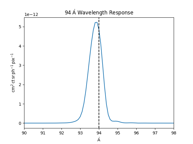
First, create the Channel object for the 94 angstrom channel and compute the wavelength response.

ch = Channel(94*u.angstrom)
correction_table = get_correction_table("jsoc")
response = ch.wavelength_response(correction_table=correction_table)
response *= ch.plate_scale

Files Downloaded:   0%|          | 0/1 [00:00<?, ?file/s]

aiapy.aia_V8_all_fullinst.genx:   0%|          | 0.00/5.43M [00:00<?, ?B/s]

aiapy.aia_V8_all_fullinst.genx:   9%|▉         | 493k/5.43M [00:00<00:01, 4.33MB/s]

aiapy.aia_V8_all_fullinst.genx:  99%|█████████▉| 5.36M/5.43M [00:00<00:00, 29.0MB/s]


Files Downloaded: 100%|██████████| 1/1 [00:00<00:00,  3.73file/s]
Files Downloaded: 100%|██████████| 1/1 [00:00<00:00,  3.73file/s]

Plot the wavelength response

plt.plot(ch.wavelength, response)
plt.xlim(ch.channel + [-4, 4]*u.angstrom)
plt.axvline(x=ch.channel, ls='--', color='k')
plt.title(f'{ch.channel.to_string(format="latex")} Wavelength Response')
plt.show()

Next, we construct for the Ion object for Fe 18. Note that by default we use the coronal abundances of Feldman et al. [FMS+92].

temperature = 10.**(np.arange(4.5, 8, 0.1)) * u.K
fe18 = fiasco.Ion('Fe 18', temperature)

Compute the contribution function,

\[G(n,T,\lambda) = \mathrm{Ab}\frac{hc}{\lambda}N_{\lambda}A_{\lambda}f\frac{1}{n}\]

for each transition of Fe 18 at constant pressure of \(10^{15}\) K \(\mathrm{cm}^{-3}\). Note that we use the couple_density_to_temperature keyword such that temperature and density vary along the same axis.

constant_pressure = 1e15 * u.K * u.cm**(-3)
density = constant_pressure / fe18.temperature
g = fe18.contribution_function(density, include_protons=False,
                               couple_density_to_temperature=True)

WARNING: No rate data available for recombining ion Fe 19. Using single-ion model for Fe 18. [fiasco.ions]
2026-03-10 17:54:46 - fiasco - WARNING: No rate data available for recombining ion Fe 19. Using single-ion model for Fe 18.

Get the corresponding transition wavelengths

transitions = fe18.transitions.wavelength[fe18.transitions.is_bound_bound]
energy = const.h * const.c / transitions / u.photon

Interpolate the response function to the transition wavelengths

f = interp1d(ch.wavelength, response, fill_value='extrapolate')
response_transitions = f(transitions) * response.unit

In order to compute the temperature response function \(K_c\), we integrate the wavelength response function \(R_c\), weighted by the contribution function \(G(\lambda,T)\), over wavelength,

\[K_c(T) = \int_0^{\infty}\mathrm{d}\lambda\,G(\lambda,T)R_c(\lambda)\]

We divide by \(hc/\lambda\) in order to convert from units of energy to photons. For more more information on the AIA wavelength response calculation, see Boerner et al. [BEL+12].

K = (g / energy * response_transitions).sum(axis=2) / (4*np.pi*u.steradian)
K = K.squeeze().to('cm5 DN pix-1 s-1')

Plot the effective temperature response function for the 94 channel.

plt.plot(temperature, K)
plt.xscale('log')
plt.yscale('log')
plt.ylim(1e-29, 1e-26)
plt.xlim(1e5, 3e7)
plt.title(f'{ch.channel.to_string(format="latex")} Response for {fe18.ion_name_roman}')
plt.show()

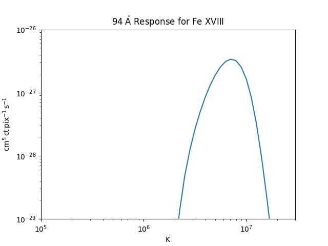
Note that this represents only the contribution of Fe 18 to the 94 angstrom bandpass. In order to construct the full response functions, one would need to repeat this procedure for every ion listed in the CHIANTI atomic database and for all AIA channels.