Creating an IonCollection

This example shows how to create an IonCollection object.

import astropy.units as u
import matplotlib.pyplot as plt
import numpy as np

from astropy.visualization import quantity_support

import fiasco

# sphinx_gallery_thumbnail_number = 2

quantity_support()

<astropy.visualization.units.quantity_support.<locals>.MplQuantityConverter object at 0x7f5c9af540d0>

The IonCollection object allows you to create arbitrary collections of Ion objects. This provides an easy way to compute quantities that combine emission from multiple ions, such as a spectra or a radiative loss curve.

We will create IonCollection containing both O VI and Fe XVIII

temperature = np.geomspace(1e4,1e8,100) * u.K
fe18 = fiasco.Ion('Fe XVIII', temperature)
o6 = fiasco.Ion('O VI', temperature)
col = fiasco.IonCollection(fe18, o6)
print(col)

Ion Collection
--------------
Number of ions: 2
Temperature range: [0.010 MK, 100.000 MK]

Available Ions
--------------
Fe 18
O 6

The only requirement for ions in the same collection is that they use the same temperature array. We can also index our collection in the same manner as a Element object to access the individual ions.

print(col[0])

CHIANTI Database Ion
---------------------
Name: Fe 18
Element: iron (26)
Charge: +17
Number of Levels: 337
Number of Transitions: 7712

Temperature range: [0.010 MK, 100.000 MK]

HDF5 Database: /home/docs/.fiasco/chianti_dbase.h5
Using Datasets:
  ioneq: chianti
  abundance: sun_coronal_1992_feldman_ext
  ip: chianti

Or iterate through them.

for ion in col:
    print(ion.ion_name_roman)

Fe XVIII
O VI

You can also create a collection using the addition operator. This is equivalent to using the IonCollection constructor as we did above.

col = fe18 + o6

Furthermore, you can iteratively build a collection in this way as well. For example, to create a new collection that includes Fe XV from the collection we created above,

new_col = col + fiasco.Ion('Fe XV', temperature)
print(new_col)

Ion Collection
--------------
Number of ions: 3
Temperature range: [0.010 MK, 100.000 MK]

Available Ions
--------------
Fe 18
O 6
Fe 15

You can even add Element objects as well, which results in every ion of that element being added to your collection.

new_col = col + fiasco.Element('carbon', temperature)
print(new_col)

Ion Collection
--------------
Number of ions: 9
Temperature range: [0.010 MK, 100.000 MK]

Available Ions
--------------
Fe 18
O 6
C 1
C 2
C 3
C 4
C 5
C 6
C 7

There are several methods on IonCollection for easily computing quantities with contributions from multiple ions. As an example, let’s compute the radiative loss for our collection containing Fe XVIII and O VI.

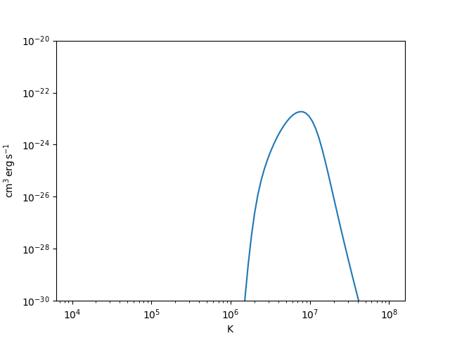
First, let’s create an IonCollection containing just Fe XVIII.

col = fiasco.IonCollection(fe18)

Now, let’s compute the radiative loss as a function of temperature for just Fe XVIII

density = 1e9*u.cm**(-3)
rl = col.radiative_loss(density)
plt.plot(col.temperature, rl)
plt.yscale('log')
plt.xscale('log')
plt.ylim(1e-30, 1e-20)

WARNING: No proton data available for Fe 18. Not including proton excitation and de-excitation in level populations calculation. [fiasco.ions]

(1e-30, 1e-20)

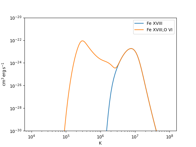
Next, let’s add O VI and again compute the radiative loss.

new_col = fe18 + o6
rl_new = new_col.radiative_loss(density)
plt.plot(col.temperature, rl, label=','.join([i.ion_name_roman for i in col]))
plt.plot(new_col.temperature, rl_new, label=','.join([i.ion_name_roman for i in new_col]))
plt.yscale('log')
plt.xscale('log')
plt.ylim(1e-30, 1e-20)
plt.legend()

WARNING: No proton data available for Fe 18. Not including proton excitation and de-excitation in level populations calculation. [fiasco.ions]
WARNING: No proton data available for O 6. Not including proton excitation and de-excitation in level populations calculation. [fiasco.ions]

<matplotlib.legend.Legend object at 0x7f5c9b1dd690>

By comparing the radiative losses, we can clearly see at what temperatures the respective ions are dominating.