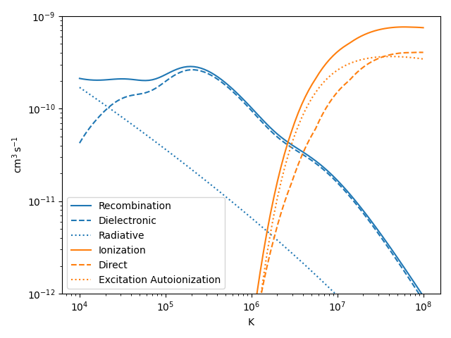
Ionization and recombination rates

This example shows how to compute the recombination rate as a function of temperature for Fe 16, including the radiative and dielectronic components.

import astropy.units as u
import matplotlib.pyplot as plt
import numpy as np

from astropy.visualization import quantity_support

from fiasco import Ion

quantity_support()

<astropy.visualization.units.quantity_support.<locals>.MplQuantityConverter object at 0x7f5c9b12b150>

First, instantiate the Fe XVI ion object. This can be done in a number of ways, but we will use the spectroscopic roman numeral notation.

ion = Ion('Fe XVI', np.logspace(4, 8, 100) * u.K)

We can calculate the recombination rate, which includes contributions from both radiative and dielectronic recombination. We can also compute these separately in order to understand over what temperature range each process dominates. Similarly, we can calculate the ionization rate which includes contributions from direction ionization and excitation autoionization. We can plot the recombination and ionization rates, including all components, as a function of temperature.

fig, ax = plt.subplots(tight_layout=True)
ax.plot(ion.temperature, ion.recombination_rate,
        label='Recombination', color='C0',)
ax.plot(ion.temperature, ion.dielectronic_recombination_rate,
        label='Dielectronic', color='C0', ls='--')
ax.plot(ion.temperature, ion.radiative_recombination_rate,
        label='Radiative', color='C0', ls=':')
ax.plot(ion.temperature, ion.ionization_rate,
        label='Ionization', color='C1')
ax.plot(ion.temperature, ion.direct_ionization_rate,
        label='Direct', color='C1', ls='--')
ax.plot(ion.temperature, ion.excitation_autoionization_rate,
        label='Excitation Autoionization', color='C1', ls=':')
ax.set_xscale('log')
ax.set_yscale('log')
ax.set_ylim(1e-12, 1e-9)
ax.legend()
plt.show()