Non-equilibrium Ionization

In this example, we’ll show how to compute the ionization fractions of iron in the case where the the timescale of the temperature change is shorter than the ionization timescale. This is often referred to as non-equilibrium ionization.

import astropy.units as u
import matplotlib.pyplot as plt
import numpy as np

from astropy.visualization import quantity_support
from scipy.interpolate import interp1d

from fiasco import Element

# sphinx_gallery_thumbnail_number = 3

quantity_support()

<astropy.visualization.units.quantity_support.<locals>.MplQuantityConverter object at 0x7f5c9048e150>

The time evolution of an ion fraction \(f_k\) for some ion \(k\) for some element is given by,

\[\frac{d}{dt}f_k = n_e(\alpha_{k-1}^I f_{k-1} + \alpha_{k+1}^R f_{k+1} - \alpha_{k}^I f_k - \alpha_k^R f_k),\]

where \(n_e\) is the electron density, \(\alpha^I\) is the ionization rate, and \(\alpha^R\) is the recombination. Both the ionization and recombination rates are a function of electron temperature \(T_e\).

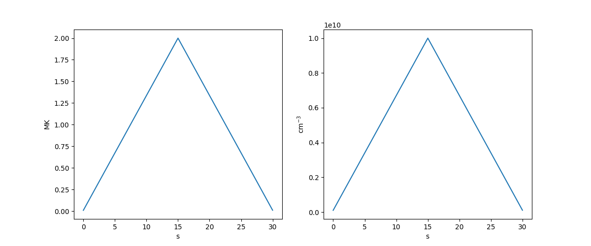
Consider a very simple temperature evolution model in which the electron temperature rises from \(10^4\) K to \(1.5\times10^7\) K over 15 s and then decreases back to \(10^4\) K.

t = np.arange(0, 30, 0.01) * u.s
Te_min = 1e4 * u.K
Te_max = 2e6 * u.K
t_mid = 15 * u.s
Te = Te_min + (Te_max - Te_min) / t_mid * t
Te[t>t_mid] = Te_max - (Te_max - Te_min) / t_mid * (t[t>t_mid] - t_mid)

Similarly, we’ll model the density as increasing from \(10^8\,\mathrm{cm}^{-3}\) to \(1.5^10\,\mathrm{cm}^{-3}\) and then back down to \(10^8\,\mathrm{cm}^{-3}\).

ne_min = 1e8 * u.cm**(-3)
ne_max = 1e10 * u.cm**(-3)
ne = ne_min + (ne_max - ne_min) / t_mid * t
ne[t>t_mid] = ne_max - (ne_max - ne_min) / t_mid * (t[t>t_mid] - t_mid)

We can plot the temperature and density as a function of time.

plt.figure(figsize=(12,5))
plt.subplot(121)
plt.plot(t,Te.to('MK'))
plt.subplot(122)
plt.plot(t,ne)
plt.show()

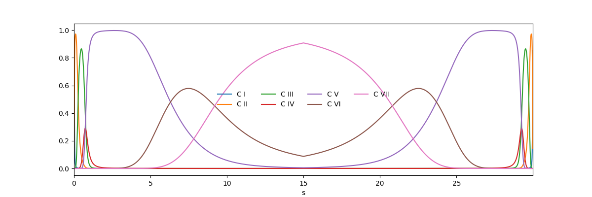
In the case where the ionization fraction is in equilibrium, the left hand side of the above equation is zero. As shown in previous examples, we can get the ion population fractions of any element in the CHIANTI database over some temperature array with equilibrium_ionization. First, let’s model the ionization fractions of C for the above temperature model, assuming ionization equilibrium.

temperature_array = np.logspace(4, 8, 1000) * u.K
carbon = Element('carbon', temperature_array)
func_interp = interp1d(carbon.temperature.to_value('K'), carbon.equilibrium_ionization.value,
                       axis=0, kind='cubic', fill_value='extrapolate')
carbon_ieq = u.Quantity(func_interp(Te.to_value('K')))

We can plot the population fractions as a function of time.

plt.figure(figsize=(12, 4))
for ion in carbon:
    plt.plot(t, carbon_ieq[:, ion.charge_state], label=ion.ion_name_roman)
plt.xlim(t[[0,-1]].value)
plt.legend(ncol=4, frameon=False)
plt.show()

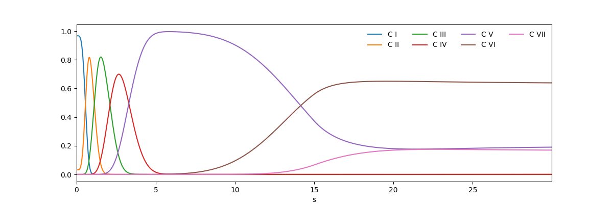
Now, let’s compute the population fractions in the case where the population fractions are out of equilibrium. We solve the above equation using the implicit method outlined in Appendix A of Barnes et al. [BBV19],

\[\mathbf{F}_{l+1} = \left(\mathbb{I} - \frac{\delta}{2}\mathbf{A}_{l+1}\right)^{-1}\left(\mathbb{I} + \frac{\delta}{2}\mathbf{A}_l\right)\mathbf{F}_l\]

where \(\mathbf{F}_l\) is the vector of population fractions of all states at time \(t_l\), \(\mathbf{A}_l\) is the matrix of ionization and recombination rates with dimension \(Z+1\times Z+1\) at time \(t_l\), and \(\delta\) is the time step.

First, we can set our initial state to the equilibrium populations.

carbon_nei = np.zeros(t.shape + (carbon.atomic_number + 1,))
carbon_nei[0, :] = carbon_ieq[0,:]

Then, interpolate the rate matrix to our modeled temperatures

func_interp = interp1d(carbon.temperature.to_value('K'), carbon._rate_matrix.value,
                       axis=0, kind='cubic', fill_value='extrapolate')
fe_rate_matrix = func_interp(Te.to_value('K')) * carbon._rate_matrix.unit

Finally, we can iteratively compute the non-equilibrium ion fractions using the above equation.

identity = u.Quantity(np.eye(carbon.atomic_number + 1))
for i in range(1, t.shape[0]):
    dt = t[i] - t[i-1]
    term1 = identity - ne[i] * dt/2. * fe_rate_matrix[i, ...]
    term2 = identity + ne[i-1] * dt/2. * fe_rate_matrix[i-1, ...]
    carbon_nei[i, :] = np.linalg.inv(term1) @ term2 @ carbon_nei[i-1, :]
    carbon_nei[i, :] = np.fabs(carbon_nei[i, :])
    carbon_nei[i, :] /= carbon_nei[i, :].sum()

carbon_nei = u.Quantity(carbon_nei)

And plot the non-equilibrium populations as a function of time

plt.figure(figsize=(12,4))
for ion in carbon:
    plt.plot(t, carbon_nei[:, ion.charge_state], ls='-', label=ion.ion_name_roman,)
plt.xlim(t[[0,-1]].value)
plt.legend(ncol=4, frameon=False)
plt.show()

We can compare the two equilibrium and non equilbrium cases directly by overplotting the C V population fractions for the two cases.

plt.figure(figsize=(12,4))
plt.plot(t, carbon_ieq[:, 4], label='IEQ')
plt.plot(t, carbon_nei[:, 4], label='NEI',)
plt.xlim(t[[0,-1]].value)
plt.legend(frameon=False)
plt.show()

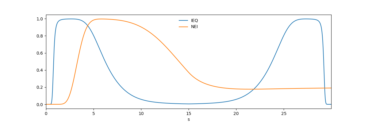
Note that the equilibrium populations exactly track the temperature evolution while the peak of the non-equilibrium Fe XVI population lags the equilibrium case and is not symmetric.

Finally let’s plot the effective temperature as described in Bradshaw [Bra09]. Qualitatively, this is the temperature that one would infer if they observed the non-equilibrium populations and assumed the populations were in equilibrium.

Te_eff =  carbon.temperature[[(np.fabs(carbon.equilibrium_ionization - carbon_nei[i, :])).sum(axis=1).argmin()
                          for i in range(carbon_nei.shape[0])]]
plt.plot(t, Te.to('MK'), label=r'$T$')
plt.plot(t, Te_eff.to('MK'), label=r'$T_{\mathrm{eff}}$')
plt.xlim(t[[0,-1]].value)
plt.legend()
plt.show()

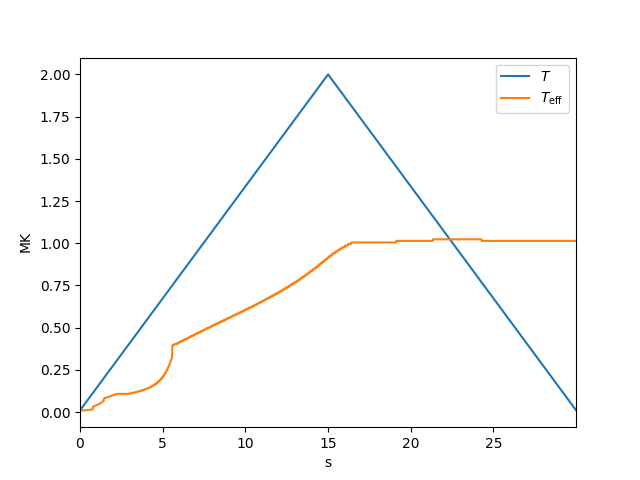
Note that the effective temperature is consistently less than the actual temperature, emphasizing the point that non-equilibrium ionization makes it difficult to detect very hot plasma when the temperature changes rapidly and/or the density is low.